")
Database statistics are a powerful weapon. They store a vast array of information about the database data that helps identify slow-running queries and allows you to devise an algorithm to optimize query execution. The query optimizer embedded in your SQL Server database uses statistical data to tune execution plans according to the way your data characteristics change. That is why it is vital to keep the statistics up to date and to understand them well. Therefore, in this article, we are going to look at how to collect statistical information and how to interpret it correctly.
What is DBCC SHOW_STATISTICS Command
DBCC SHOW_STATISTICS shows the current query optimization statistics for a table or indexed view. Simply put, the command allows us to view the statistics that SQL Server will use to create a high-quality query plan. In fact, the query optimizer uses the statistics to opt for a better query plan, such as choosing the index seek operator instead of the index scan operator to enhance query performance by eliminating a resource-heavy index scan.
Syntax
DBCC SHOW_STATISTICS statement returns three data sets: the header, density vector, and histogram. The syntax for the command is as follows:
DBCC SHOW_STATISTICS (‘Object_Name’, ‘Target’)You can specify a table or indexed view as an object and statistics or an index as a target. Running the above-mentioned command will output a result consisting of all three sections. If you need to retrieve a specific data set (for instance, the histogram), you can specify a required argument in the syntax:
DBCC SHOW_STATISTICS (‘Object_Name’, ‘Statistic_Name’) WITH HISTOGRAM;or
DBCC SHOW_STATISTICS (‘Object_Name’, ‘Statistic_Name’) WITH STAT_HEADER;or
DBCC SHOW_STATISTICS (‘Object_Name’, ‘Statistic_Name’) WITH DENSITY_VECTOR;Example
In the example below, we executed the DBCC SHOW_STATISTICS statement, and we received the three sections (the header, density vector, and histogram) in the output, as follows:
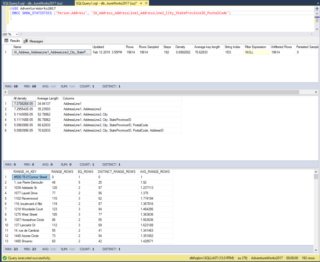
DBCC SHOW_STATISTICS Statistics Header
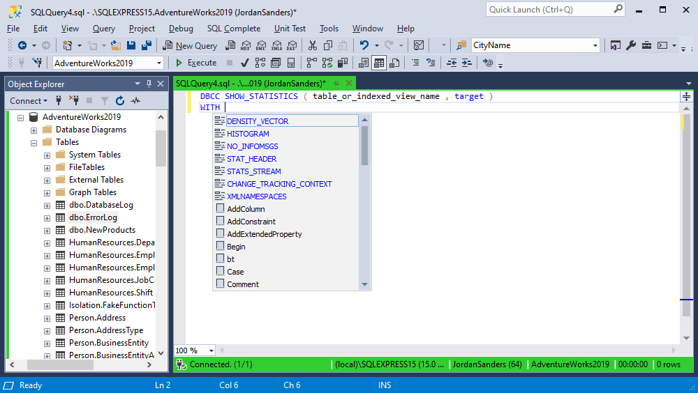
To understand each section better, let’s take a closer look at the information it delivers. We can modify the previous statement to limit the result set to the header. Using the auto-completion feature of SQL Complete add-in from dbForge Studio, we can easily specify the necessary argument:
Let’s execute the query as follows:
USE AdventureWorks2017DBCC SHOW_STATISTICS ('Person.Address', 'IX_Address_AddressLine1_AddressLine2_City_StateProvinceID_PostalCode') WITH STAT_HEADER;The output displays the following information:
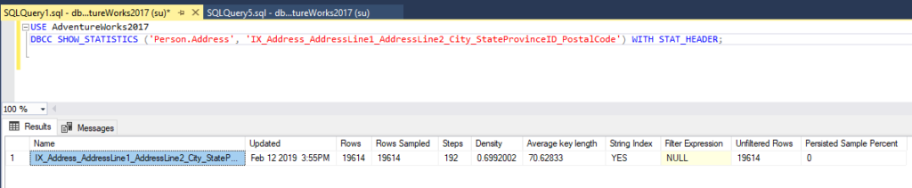
When STAT_HEADER is defined, the information returned in the result set displays general information about the statistics:
| Column Name | Description |
| Name | The name of the statistics. |
| Updated | The date and time of the most recent update of the statistics. You can also retrieve this information by running the STATS_DATE system function. |
| Rows | The total number of rows in the table or indexed view as of the most recent update of the statistics. |
| Rows Sampled | The number of rows that were selected to create the statistics. |
| Steps | The number of steps within the histogram. |
| Density | This value is no longer used by the Query Optimizer, and it is shown for the purpose of backward compatibility. |
| Average Key Length | The average of bytes per value for all of the key columns in the statistics. |
| String Index | YES states that the statistics comprise string summary statistics used to enhance cardinality estimates for the queries with the LIKE operator. |
| Filter Expression | If the statistics are filtered, the filter predicate is shown. If they are not filtered, the result is set to NULL. |
| Unfiltered Rows | The total number of rows before the filter expression was applied. |
| Persisted Sample Percent | The persisted sample percentage used for statistics updates. |
DBCC SHOW_STATISTICS Density Vector
The next section is the density vector. It represents the level of unique values present within a column or multiple columns of the statistics. The density vector is calculated according to the following formula: 1 / number of distinct values. The example below has six levels for the density vector: the first is computed for column one, the second for columns one and two, the third refers to columns one, two, and three, and so on. Let’s execute the following query:
USE AdventureWorks2017
DBCC SHOW_STATISTICS ('Person.Address', 'IX_Address_AddressLine1_AddressLine2_City_StateProvinceID_PostalCode') WITH DENSITY_VECTOR;
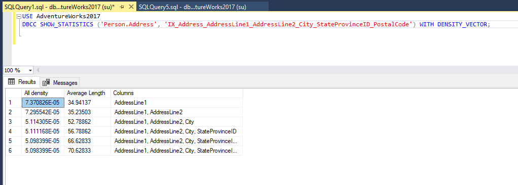
Note that DBCC SHOW STATISTICS uses the E notation to reduce the number length to 7.370826E-05, which can be converted to 0,00007370826. This number is very close to zero, which indicates that the values stored in the AddressLine1 are almost all unique.
| Column Name | Description |
| All Density | Density is calculated as 1/n where n is the number of distinct values in a column or a group of columns. The closer the Density is to zero, the more unique is the key value, that’s why the last row (6) has the lowest density. |
| Average Length | The average size (measured in bytes) of the column or set of columns that make up the statistics. |
| Columns | The names of columns in the table for which All density and Average length are displayed. |
DBCC SHOW_STATISTICS Histogram
A histogram specifies how often a distinct column value occurs across a data set. The data set is represented as a fixed number of intervals, known as steps, that can reach 200. In order to generate a histogram, the query optimizer sorts the column values, calculates the number of values that match every distinct column value, and then puts the column values together into a maximum of 200 steps. Each step contains a column range that is followed by an upper bound column value. To view a histogram, execute the following query:
USE AdventureWorks2017
DBCC SHOW_STATISTICS ('Person.Address', 'IX_Address_AddressLine1_AddressLine2_City_StateProvinceID_PostalCode') WITH HISTOGRAM;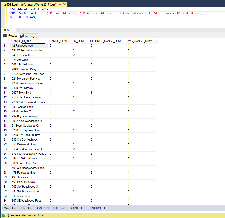
Let’s clarify the columns of the histogram:
| Column Name | Description |
| RANGE_HI_KEY | The highest column value for a histogram step. |
| RANGE_ROWS | The number of rows used in a histogram step. |
| EQ_ROWS | The number of rows that equals RANGE_HI_KEY column value in a histogram step. |
| DISTINCT_RANGE_ROWS | The number of rows that contain distinct column values within a histogram step. |
| AVG_RANGE_ROWS | The average number of rows that contain duplicate column values. It is calculated by dividing RANGE_ROWS by DISTINCT_RANGE_ROWS when DISTINCT_RANGE_ROWS exceeds zero, otherwise, its value is 1. |
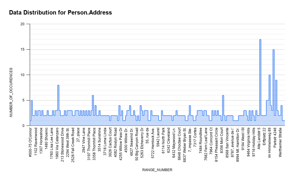
For learning purposes, you can build an Excel graphic based on the retrieved values. The image below is the representation of the data distribution on the Person.Address table from the AdventureWorks2017 database that is based on the histogram of the IX_Address_AddressLine1_AddressLine2_City_StateProvinceID_PostalCode statistics. The x-axis represents a value for the AddressLine1 column of the Person.Address table and the y-axis is the number of occurrences of that value.
How Statistics Affect Plan Generation
Using the statistics, we obtained the necessary information, such as the structure of data in the Person.Address table and defined how effective querying of PK_Address_AddressID index would be. Now, we can create and execute two queries against the database: where one query will apply an index scan, and the other one will use a full table scan. Consider the Person.Address table and the PK_Address_AddressID histogram.
First, let’s run the query in which we select the values from the neighboring cells of the Person.Address table:
SELECT * FROM [Person].[Address] WHERE AddressLine1 BETWEEN '2876 Bayview Ct' AND '2031 Fox Hill Loop';As you see from the query execution plan below, the table scan will be used to execute the query:
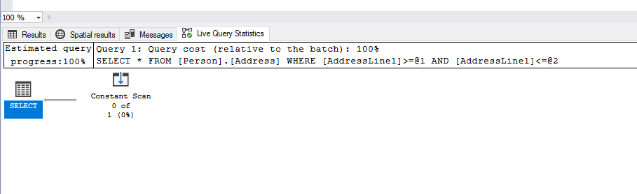
That’s because the query contains the predicate BETWEEN ‘2876 Bayview Ct’ AND ‘2031 Fox Hill Loop’, and it needs to retrieve a small amount of data from the table.
This time let’s run the SELECT statement and specify the values that are far from one other:
SELECT * FROM [Person].[Address] WHERE AddressLine1 BETWEEN '342 Old Oak Highway' AND '867 SE Hazelwood Road';In this case, the index scan will be used:
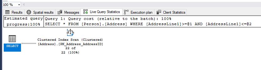
That’s because in this query, the predicate BETWEEN ‘342 Old Oak Highway’ AND ‘867 SE Hazelwood Road’ queries large amounts of data from the table. Thus, the obvious choice is to use the index. As you see, to get values from PK_Address_AddressID, you need to use only index scan as this index has a B-Tree Index structure.
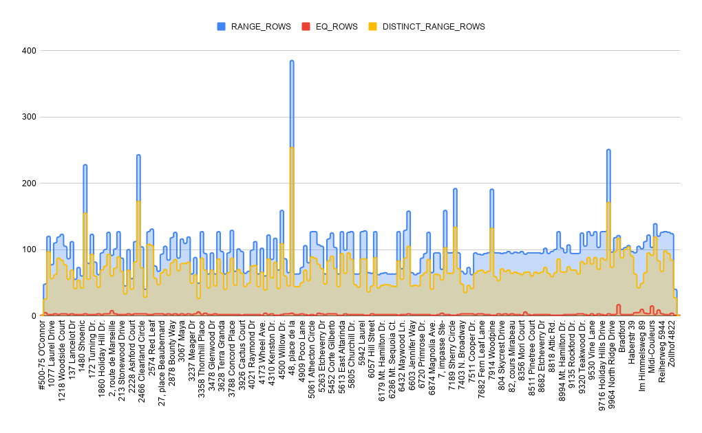
The same histogram table can be represented in a different form based on the RANGE_ROWS, EQ_ROWS, DISTINCT_RANGE_ROWS histogram columns:
Conclusion
To sum up, SQL Server query optimizer uses statistics to choose the most optimal way of querying a table. Statistics allow choosing the most effective index for frequent queries and improving their performance by selecting the optimal number of indexes and the combination of columns in them. DBAs use statistics as a method of working with and analyzing data. Such analysis involves defining the number of unique values in a column or multiple columns and identifying duplicate values, which subsequently helps to determine the effectiveness of created indexes and the ways to query data in a table more efficiently.