
TL;DR
SSIS incremental load is a technique to update data warehouses by transferring only new or modified data. This method boosts performance, reduces system load, and keeps data up to date without requiring full refreshes.
People are ever more in a hurry. They want their data almost right now. And even more, data is getting bigger and bigger. So, you can’t use good old techniques because they’re “good enough”. It has to be fast. And ETL steps are not an exemption. This is where incremental load comes to play. And if you’re on this page, you probably are looking for incremental load in SSIS.
And that’s our focus in this article. We’re going to make comparisons and examples to explain incremental data load in SSIS step-by-step. And rest assured it won’t crack your head figuring this out.
Here’s what’s in store for you:
- What are full load and incremental load in ETL?
- What is incremental data load in SSIS?
- The differences between full load and incremental load in SSIS
- Incremental load in SSIS using CDC or Change Data Capture
- Incremental load in SSIS using DateTime columns
- How to do incremental load in SSIS using Lookup
- The best tool for SSIS data loading
Each section will have subsections. You can jump to the topic you need by clicking the links.

Before we begin with the examples, let’s compare incremental load with its opposite, the full load.
What are Full Load and Incremental Load in ETL
No matter what ETL tools you use, Full and Incremental loads have the same meaning. Let’s describe them below.
Full Load in ETL
As the name suggests, Full Load in ETL is loading ALL the data from the source to the destination. A target table is truncated before loading everything from the source. That’s why this technique is also known as Destructive Load. This technique is also easier to do. And this also ensures the highest data integrity. But the size of your data today is bigger than yesterday. So, if you use this on ever-growing data, the process will get slower over time.
ETL Full Load Use Cases
- The size of the source data is small and won’t significantly grow in many years to come. Examples include a list of colors, a few categories/classifications, list of countries and cities, and many more.
- It’s hard to say which is new or changed in the source.
- Data needs to be exactly the same from the source to the destination
- The history of the data is irrelevant and is overwritten more often
Incremental Load in ETL
Meanwhile, Incremental Load is as the name suggests too. Only the data that changed will be loaded from the source to the destination. This is done incrementally over time. The ones that didn’t change will stay as-is. This is a bit difficult to do. You need to ensure that all the changes have been gathered and loaded to the destination. But this will run faster than Full Load on very large data.
ETL Incremental Load Use Cases
- Data size is very large and querying will be very slow for large result sets
- Changes are easy to query
- Deleted data needs to be retained in the destination, like an audit system
What is Incremental Load in SSIS
The basic constituents of an incremental load in SSIS are shown in Figure 1.
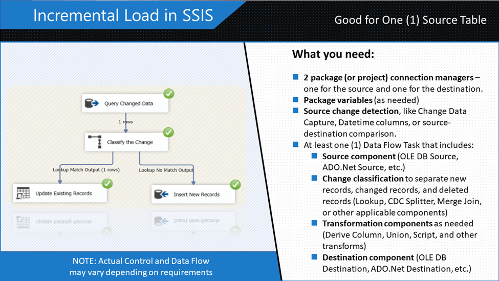
Incremental loading in SSIS tends to be more complex depending on your requirements. But the simple “recipe card” in Figure 1 includes what you need to “cook” data in increments. Capturing changes in the data is the challenging part. You can mess up the destination if you are not careful.
In the succeeding sections, you will see how to do incremental load in SSIS with examples. These include using Change Data Capture (CDC), DateTime columns, and lookups. You will also see how this is done using Devart SSIS components.
Let’s compare incremental load to full load in SSIS in the next section.
The Difference Between Full Load and Incremental Load in SSIS
You already saw what incremental load looks like in SSIS (Figure 1). Meanwhile, here’s how it goes with the SSIS Full load in Figure 2 below.
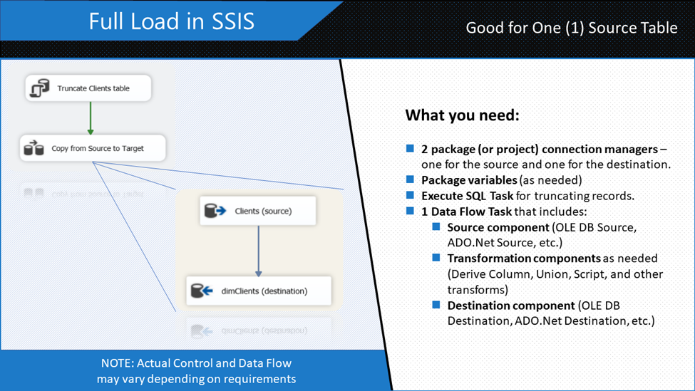
The difference between Full load and incremental load in SSIS is in the package design. A Full load design needs fewer components dragged into the SSIS package. It’s so simple there’s little thinking involved. That’s why out of a false sense of productivity, some developers tend to resort to this technique most of the time.
But running a full load design package every night is not advisable for large data, say 15TB. Do you think it will finish on time before users arrive in the morning? That won’t happen because you are trying to re-insert the records that didn’t change at all. If that is around 70% of the data, you need more downtime depending on server resources.
That’s unacceptable.
So, the more you need to use incremental load on these scenarios. In the following sections, you will learn how to load data faster using incremental load.
Incremental Load in SSIS Using CDC
First, let’s consider using Change Data Capture (CDC). Note that from here to the next 3 examples, we’re going to use simple examples. So, the package design won’t blur the objective.
Before we begin with the example, this section will cover the following:
- First, how to enable CDC in a database and table
- Then, creating the SSIS package for SSIS incremental load using CDC
- Finally, running and checking the results
Figure 3 shows the constituents of this example.
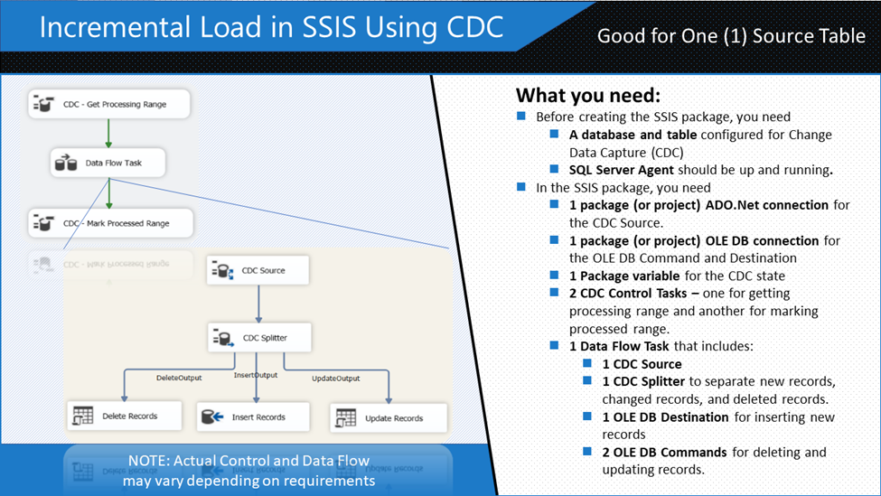
Change Data Capture (CDC) records inserts, deletes, and updates in a table. Before you can make this example work, you need a database and a table that is configured for CDC.
How to Enable CDC in a Database and Table
Database and table settings default to without CDC. To make a database CDC-enabled, here’s the T-SQL syntax:
-- point to the database you need to CDC-enable
USE SportsCarSales
GO

-- this will enable CDC to the current database.
EXEC sys.sp_cdc_enable_db
GO
Then, to check if CDC is indeed enabled, run this:
select name from sys.databases
where is_cdc_enabled=1
If the name of the database you enabled for CDC appears, you’re good to go. Your database is now CDC-enabled.
But it doesn’t end here. You need to state what table you want to track for any changes. The sp_cdc_enable_table will do the trick. Below is an example of that.
EXEC sys.sp_cdc_enable_table
@source_schema = N'dbo',
@source_name   = N'sportsCarSales',
@role_name     = NULL,
@supports_net_changes = 1
GO
Running the above code should result in similar messages below:
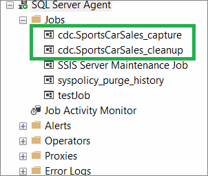
Job 'cdc.SportsCarSales_capture' started successfully.
Job 'cdc.SportsCarSales_cleanup' started successfully.
Those messages are the 2 new SQL Server Agent jobs created after enabling a table for CDC. That’s why you need SQL Server Agent to make CDC work. See a screenshot in Figure 4.
Doing inserts, deletes, and updates on the sportsCarSales table will automatically record the changes to another table named cdc.dbo_sportsCarSales_CT. This table has columns like the original. See a screenshot in Figure 5.
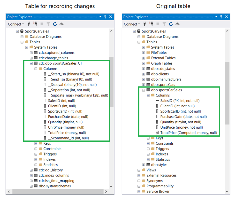
The _$operation column in the left table is of particular interest. Possible values for this column are 1 (Delete), 2 (Insert), 3, and 4 (Update). Update uses 2 values: one for column values before the update (that’s 3). And the other for column values after the update (that’s 4). You can check this column when checking the values before running your SSIS package. The CDC Source and CDC Splitter components use this table when identifying changes. More on these in the next section.
Creating the SSIS Package for SSIS Incremental Load Using CDC
Here are the steps in creating the SSIS package with incremental load using CDC. This assumes you already have a blank package in Visual Studio 2019. Our goal here is to load the rows from the sportsCarSales table into the FactSportsCarSales fact table in a data warehouse.
The following are the summary of steps:
STEP #1. Create 2 database connection managers
STEP #2. Drag 2 CDC Control Task to the Control Flow
STEP #3. Drag a Data Flow Task and Connect to the CDC Control Task
STEP #1. Create 2 Database Connection Managers
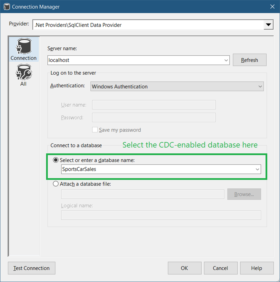
We need 2 database connections here. One is the ADO.Net connection that should point to the CDC-enabled database. And then, create an OLE DB Connection to a data warehouse as the destination. Both are SQL Server 2019 databases. See Figures 6 and 7 accordingly. In this example, both databases are on the same machine. And we’re using Windows authentication to connect.
So, in the Connection Managers window, right-click and select New ADO.Net Connection. Then, fill up the server, authentication, and database settings as seen in Figure 6 below.
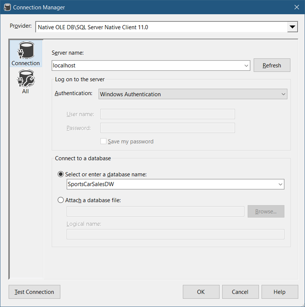
Then, create an OLE DB connection to the data warehouse. In the Connections Manager window, right-click and select New OLE DB Connection. Then, fill up the server, authentication, and database name. Specify the data warehouse here.
STEP #2. Drag 2 CDC Control Task to the Control Flow
There are 2 things we need to do after dragging a CDC Control Task in the Control Flow.
Mark CDC Start
First, we need to configure the CDC Control Task to Mark CDC Start. And then, create a CDC State table. This can be done in one configuration window. See Figure 8 below.
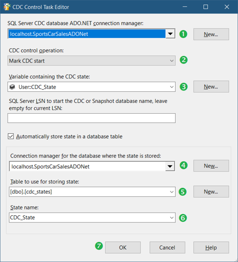
Following the numbered steps in Figure 9, the following are the details.
- Select the ADO.Net connection we created in Figure 6.
- Then, select Mark CDC start.
- Click New to create a CDC state variable. Then, a window will appear. Click OK to create the default variable name User::CDC_State.
- Select the ADO.Net connection so we can store the CDC state in that database.
- Click New to create a table for storing state. The script is already created for you. So, just click Run on the next window.
- Then, select CDC_State as the state name.
- Finally, click OK.
After configuring this CDC Control Task, run the package. You won’t see records copied to the other database yet. But the state table (dbo.cdc_state) will be populated with initial values.
From here, you can choose to disable this CDC Control Task or overwrite it again with new values in the next task.
Get Processing Range
Either you drag a new CDC Control Task to the Control Flow or overwrite the previous one. The configuration is the same as in Figure 9, except for CDC Control Operation (#2). This time, select Get processing range. Then, click OK. Connect this to the Data Flow Task in STEP #3 later.
Mark Processed Range
Configure the other CDC Control Task like the first one, except this time, select Mark processed range for the CDC Control Operation. Connect the Data Flow Task in STEP #3 to this.
Step #3. Drag a Data Flow Task and Connect to the CDC Control Task
This Data Flow Task will do the extraction and loading as seen in Figure 3 earlier. Before we dive into the details of each step, here’s a summary:
A. Add a CDC Source
B. Add a CDC Splitter and connect it to the CDC Source
C. Add an OLE DB Command to delete records
D. Add an OLE DB Destination to insert records
E. Add another OLE DB Command to update records
Now, let’s dive in.
A. Add a CDC Source
Drag a CDC Source component with settings shown in Figure 9 below.
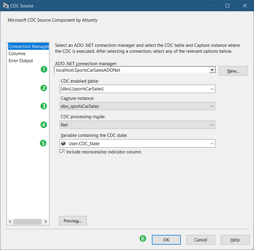
Following the numbered steps in Figure 9, the following are the details:
- First, select the ADO.Net connection we created in Figure 6.
- Then, select the CDC-enabled table sportsCarSales.
- Select the capture instance dbo_SportsCarSales.
- Then, select Net for CDC processing mode. This will return net changes only. For a detailed description of each processing mode, check out this link. You can also click Preview to see what rows will be included.
- Select the CDC State variable we created earlier (Figure 9).
- Finally, click OK.
B. Add a CDC Splitter and Connect it to the CDC Source
The only requirement of a CDC Splitter is a CDC Source preceding it. So, connect the CDC Source earlier to this component. This will separate the changes to inserts, updates, and deletes.
C. Add an OLE DB Command to Delete Records
First, you need to label this component as Delete Records (See Figure 3). Then, connect this to the CDC Splitter. When a prompt appears, select DeleteOutput for the output and click OK.
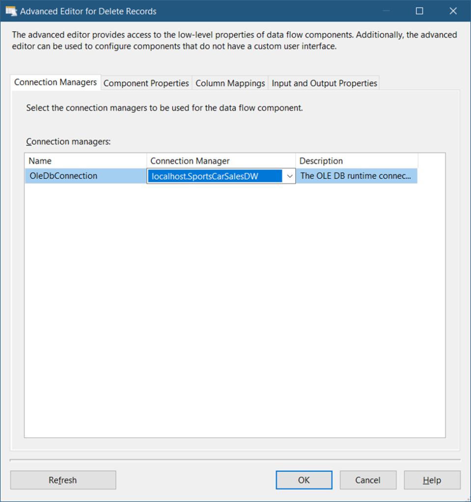
Then, configure the OLE DB Command Connection Managers tab. See Figure 10.
Next, in the Component Properties tab, specify the DELETE command for the SQLCommand property. The command should be like this:
DELETE FROM FactSportsCarSales
WHERE SalesID = ?
See a screenshot in Figure 11 below.
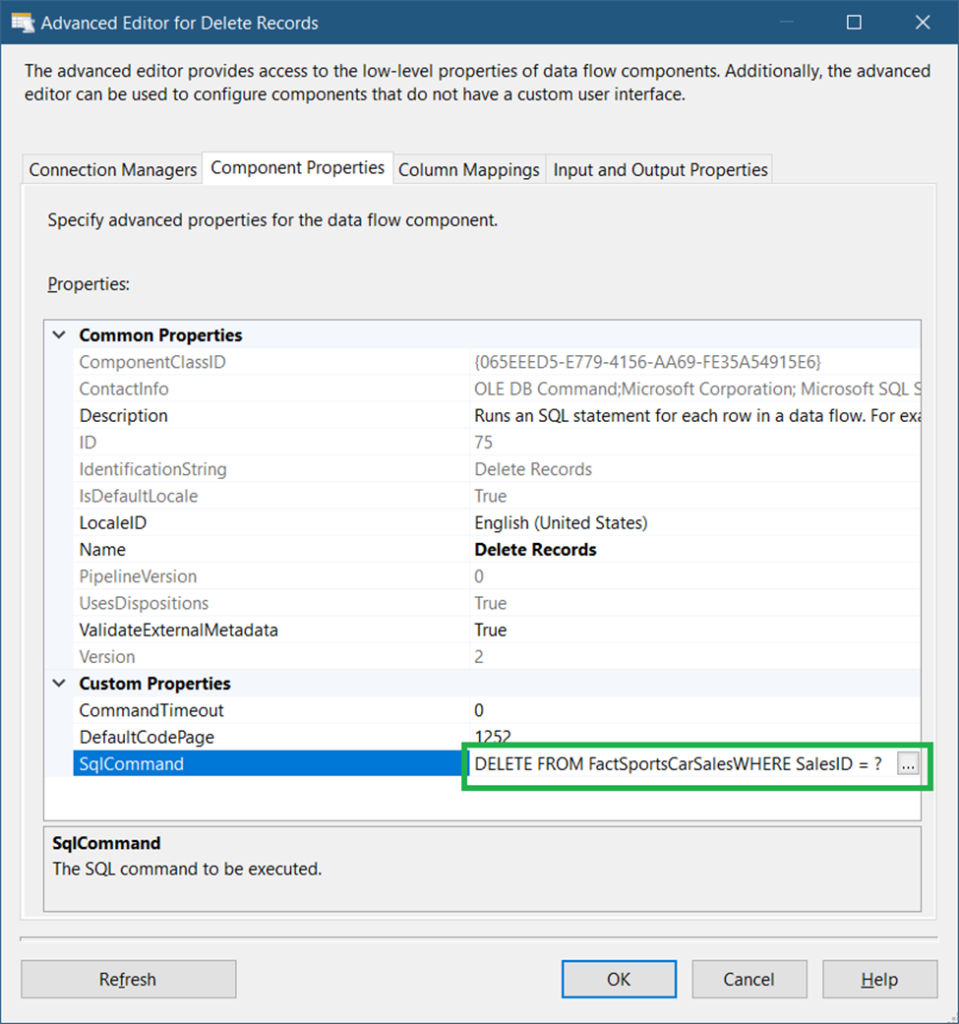
The question mark will create a parameter for SalesID. Each SalesID value coming from the CDC Splitter will be used to delete rows in the FactSportsCarSales table.
Then, in the Column Mappings tab, map the SalesID column of the table to the parameter (Param_0) See Figure 12.
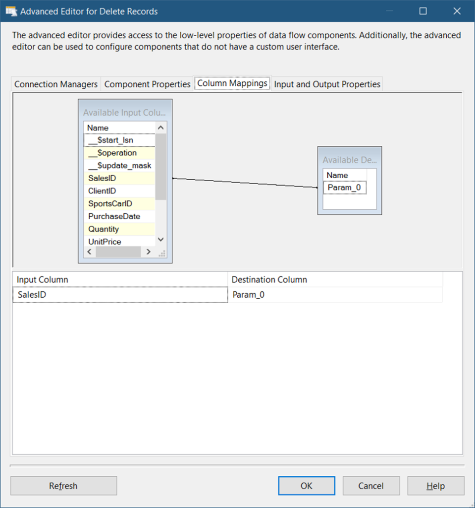
Finally, click OK.
D. Add an OLE DB Destination to Insert Records
First, drag an OLE DB Destination. Then, label it Insert Records. Connect this to the CDC Splitter. Then, select InsertOutput when a window prompt appears. See Figure 14 for the basic settings.
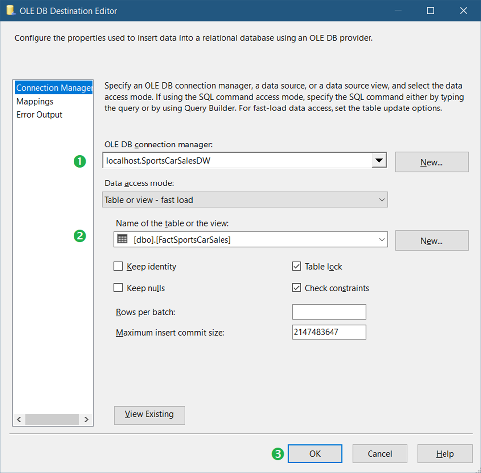
Following the numbered steps in Figure 13, below are the details:
- First, select the OLE DB Connection we created in Figure 7.
Then, select the FactSportsCarSales fact table. - Finally, click OK.
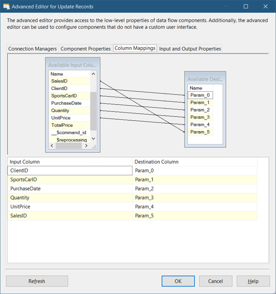
E. Add an OLE DB Command to Update Records
Drag another OLE DB Command and label it Update Records. Then, connect it to the CDC Splitter. It will automatically choose the UpdateOutput output. The Connection Managers tab setting should be the same as in Figure 11.
But the Component PropertiesSQLCommand should have a value like this:
UPDATE [dbo].[FactSportsCarSales]
   SET [ClientID] = ?
      ,[SportsCarID] = ?
      ,[PurchaseDate] = ?
      ,[Quantity] = ?
      ,[UnitPrice] = ?
 WHERE [SalesID]= ?
The number of question marks in the code above will tell you how many parameters to use starting from Param_0. The position of parameters from Param_0 to Param_5 is arranged based on their place in the code. So, Param_0 is for ClientID, Param_1 is for SportsCarID, and so on.
Check out the Column Mappings in Figure 15.
After configuring CDC in the database and table level, the way to test if CDC works is by adding and changing rows. So, let’s add some records to the table.
USE SportsCarSales
GO

INSERT INTO SportsCarSales (ClientID, SportsCarID, PurchaseDate, Quantity, UnitPrice)
	VALUES (1, 1920, '02/03/2022', 1, 845000.0000),
	(5, 1920, '01/22/2022', 1, 845000.0000),
		(54, 1920, '01/15/2022', 1, 845000.0000),
		(62, 1920, '02/04/2022', 1, 845000.0000);
GO
To see if this is recorded in CDC is by querying the cdc.dbo_sportsCarSales_CT table.
SELECT * FROM cdc.dbo_sportsCarSales_CT;Check out the results in change data capture after the INSERT command in Figure 15.
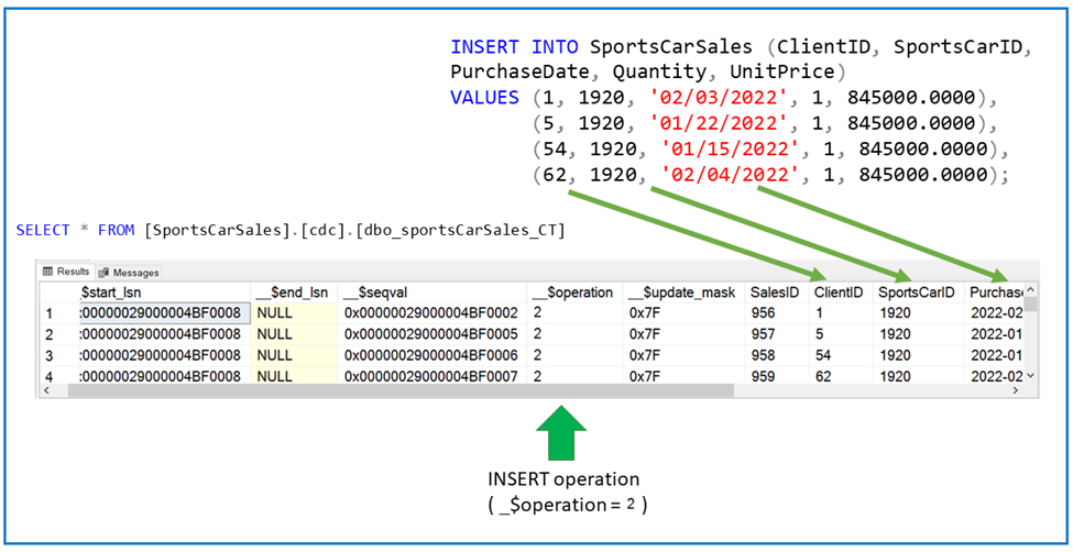
So, it did record the inserts. That’s good.
Now, try running the SSIS package earlier. The result should be the same as Figure 16 below.
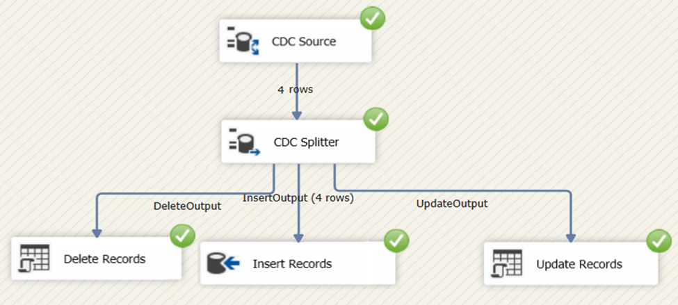
Figure 16. SSIS package runtime result for incremental load using CDC.
And finally, querying the results in the FactSportsCarSales table reveal the same set of 4 records.
Incremental Load in SSIS Using DateTime Columns
Incremental load in SSIS using DateTime columns is another way to gather data in increments. If you happen to do ETL in a table without CDC, this is your next option.
The source table may have a Modified or LastUpdate column like the one in Figure 17.
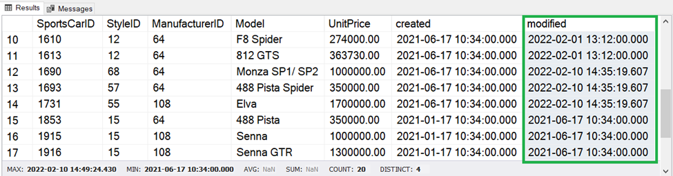
To query the changes is to know the maximum Modified column value from the destination. Then, query all records from the source that have greater than the Modified column value from the destination.
The typical ingredients of this technique are shown in Figure 18.
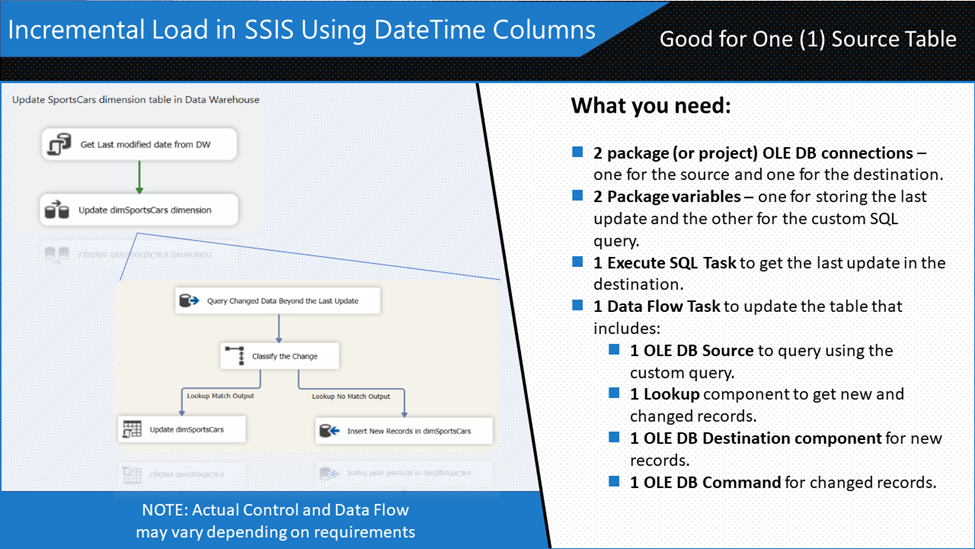
Please follow the directions on how to cook this type of incremental load. The following are the subtopics for this section:
Creating the Package to Do SSIS Incremental Load with DateTime Columns
Our objective is to load the SportsCars table into dimSportsCars dimension table in another database. The following is a summary of the steps:
STEP #1. Create 2 OLE DB connection managers
STEP #2. Create 2 package variables
STEP #3. Add an Execute SQL Task in the Control Flow
STEP #4. Add a Data Flow Task
Let’s begin.
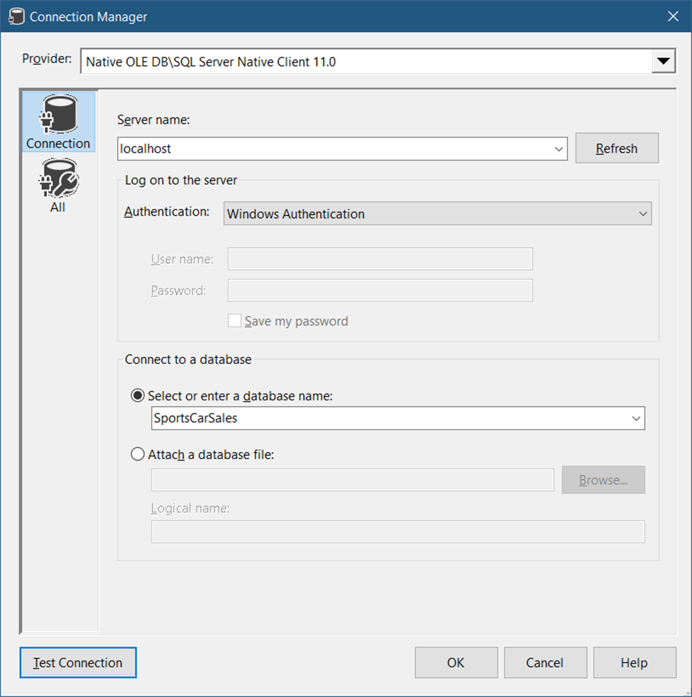
STEP #1. Create 2 OLE DB Connection Managers
The first OLE DB connection is from a transactional database. And the settings are simple as shown in Figure 19.
Then, create another OLE DB connection to the data warehouse. This should be the same as in Figure 7.
STEP #2. Create 2 Package Variables
The first variable will hold the last modified date from the dimSportsCars dimension table. Then, the second will hold the custom SQL query.
A. Create the User::sportsCars_lastUpdate Variable
- In the Variables window, click Add variable.
- Name it sportsCars_lastupdate.
- Set the data type to DateTime.
B. Create the User::sqlCommand Variable
- In the Variables window, click Add variable.
- Name it sqlCommand.
- Set the type to String.
- Click the ellipsis button to create the Expression. See Figure 21 for the Expression Builder window and the actual string expression.
- Click OK.
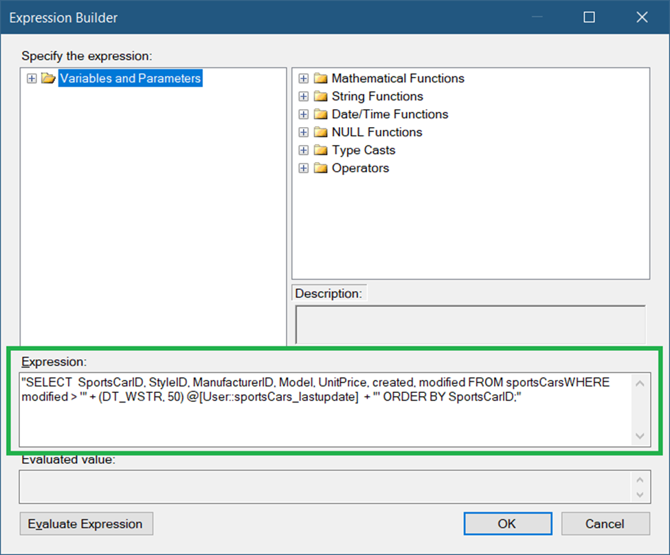
The SQL string should be like this:
"SELECT  SportsCarID, StyleID, ManufacturerID, Model, UnitPrice, created, modified
FROM sportsCars
WHERE modified > '" + (DT_WSTR, 50) @[User::sportsCars_lastupdate]  + "'
ORDER BY SportsCarID;"
Notice that we set the WHERE clause to Modified greater than User::sportsCars_lastupdate.
There will be more details about setting the 2 variables in the succeeding steps.
STEP #3. Add an Execute SQL Task in the Control Flow
This task will query the destination table to get the last Modified date value. Drag an Execute SQL Task to the Control Flow. Then, label it Get Last Modified Date from DW. Then, see the settings in Figure 21.
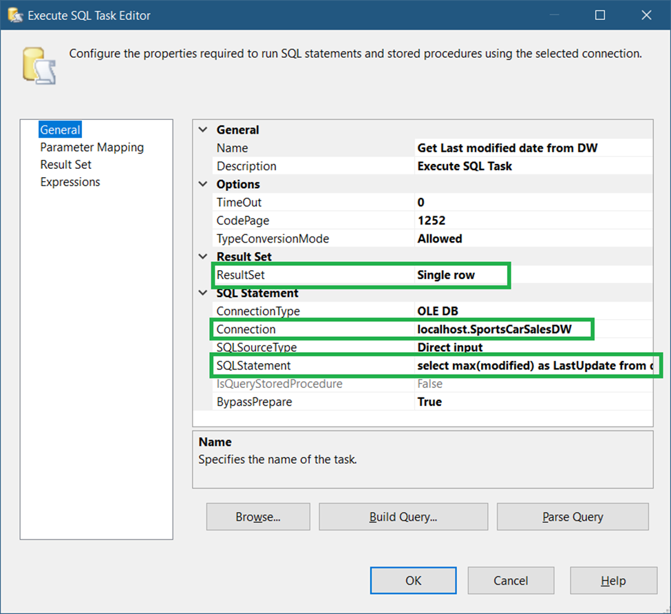
The important properties to set here are the Connection, SQLStatement, and ResultSet properties.
Set the Connection property to the second OLE DB connection set in STEP #1. Then, set the SQLStatement property to the code below.
select max(modified) as LastUpdate from dimSportsCarsThen, set the ResultSet property to a Single row.
Finally, you need to map the LastUpdate column alias (see code above) to the User::sportsCars_lastupdate variable. See a screenshot in Figure 22.
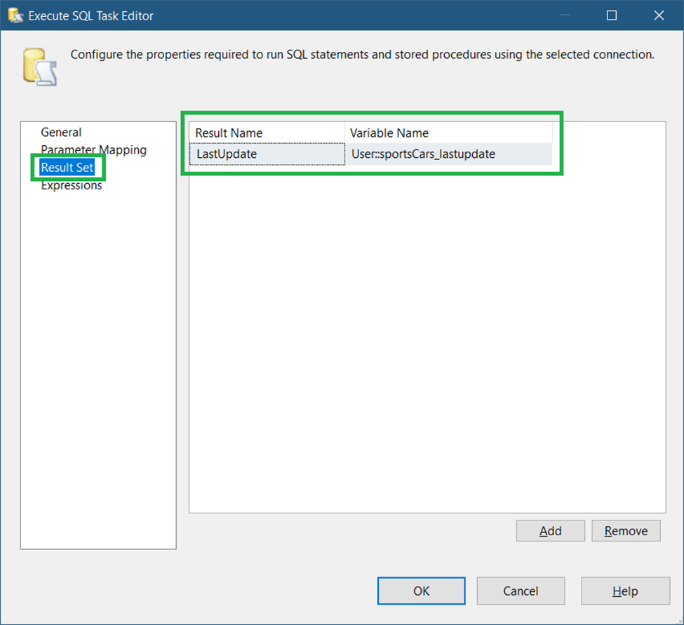
Finally, click OK to save the new settings.
STEP #4. Add a Data Flow Task
Drag a Data Flow Task to the Control Flow and connect the Execute SQL Task to it. Then, label the Data Flow Task Update dimSportsCars dimension. Then, follow the steps to add components to the Data Flow Task.
The Data Flow Task has several steps within it:
A. Add an OLE DB Source
B. Add a Lookup Transformation to compare the source to the destination
C. Add an OLE DB Command to update records
D. Add an OLE DB Destination to insert records
Now, let’s begin.
A. Add an OLE DB Source
This OLE DB Source will query the source table for the changed records. See the settings in Figure 23.

Following the numbers in Figure 23, here are the details:
- First, specify the OLE DB connection we created. See Figure 20.
- Then, set the Data access mode to SQL command from the variable.
- Then, select the variable User::sqlCommand that we created earlier. See Figure 21.
- Finally, click OK.
B. Add a Lookup Transformation to Compare the Source to the Destination
Now, we need to have a way to compare the source and the destination tables. We can use the Lookup Transformation component to do that. This will perform a join between the 2 tables.
So, drag a Lookup Transformation in the Data Flow and name it Classify the Change. Then, connect it to the OLE DB Source earlier. Double-click it. See Figure 24 for setting up the General page.
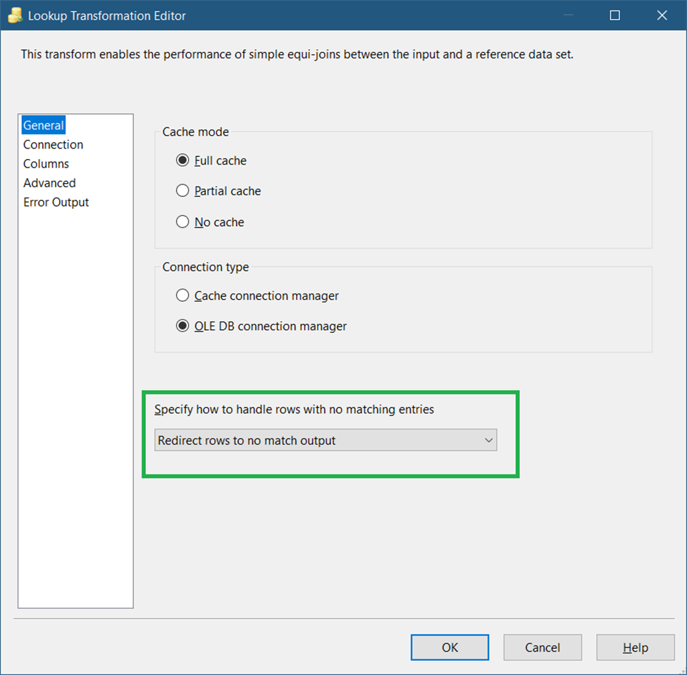
Set the dropdown to Redirect rows to no match output as seen in Figure 24. This means we are going to use the rows that have no match. And in this case, this is for detecting rows present in the source but not in the destination.
Next, click the Connection page in the left pane of the Lookup Transformation Editor. Then, see Figure 25 on what to set.

In Figure 26, you need to specify the OLE DB Connection for the target table. (See Figure 7). And then, set the SQL query to the code below.
SELECT SportsCarID from dimSportsCarsWe only need the SportsCarID column to compare, so we used a query instead of the whole table.
Next, click the Columns page to set the mapping of the source query key column to the destination. See Figure 26 for the mapping.
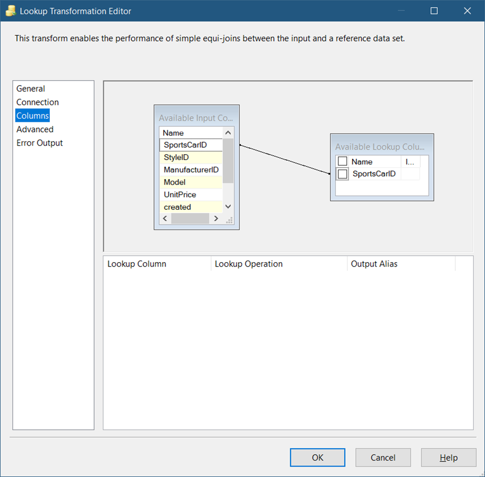
As seen in Figure 26, there should be a line from the source to the destination using the SportsCarID key column. Both key columns will be used for the comparison.
Finally, click OK.
C. Add an OLE DB Command to Update Records
This part will update the records that have matching SportsCarID key values from the Lookup Transformation.
So, drag an OLE DB Command in the Data Flow and name it Update dimSportsCars. Then, connect it to the Lookup Transformation earlier. When a prompt appears, set the Output to Lookup Match Output. Then, click OK.
Double-click the OLE DB Command and set the properties in the Connection Managers tab. See Figure 27.
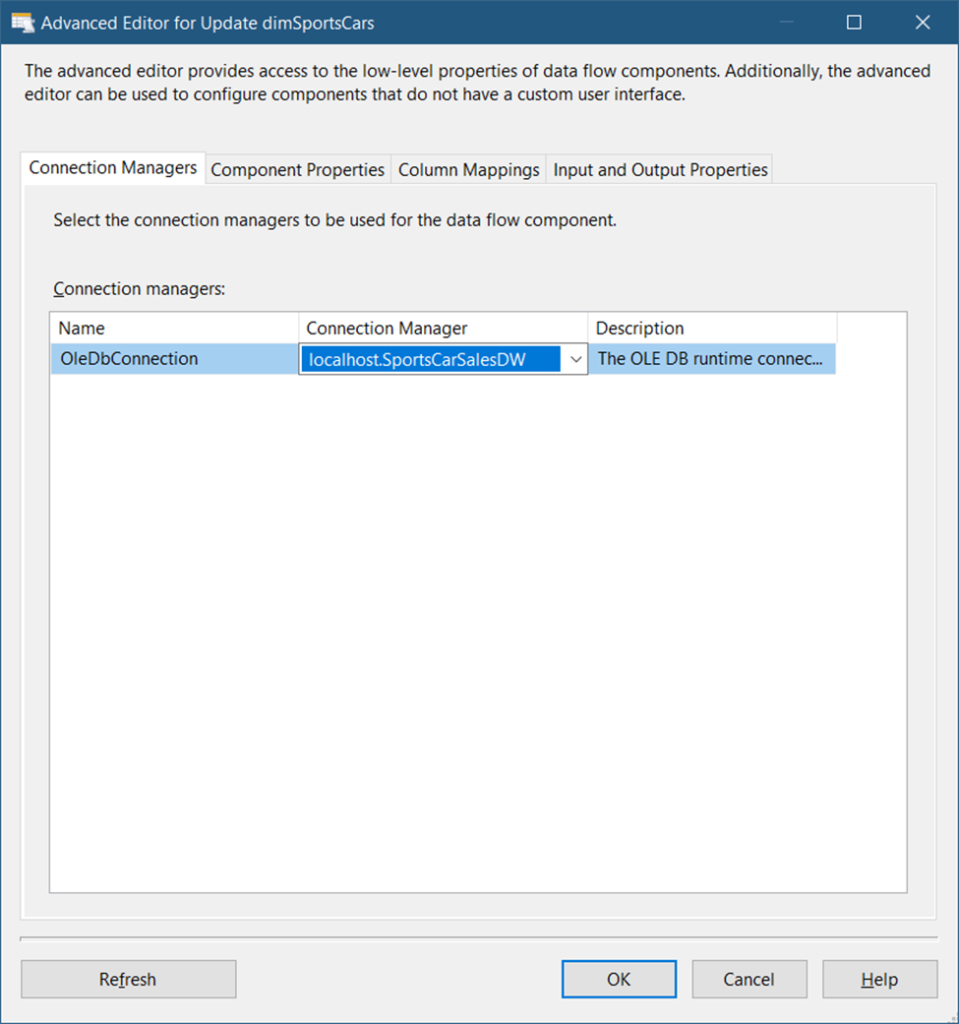
Figure 27 shows that you need to set the Connection Manager to the target database (See Figure 8). Then, click the Component Properties tab. See Figure 28 for the property settings.
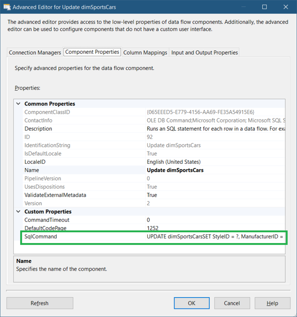
The SQLCommand property is set to:
UPDATE dimSportsCars
SET StyleID = ?, ManufacturerID = ? , MODEL = ? , UnitPrice = ? , modified = ?
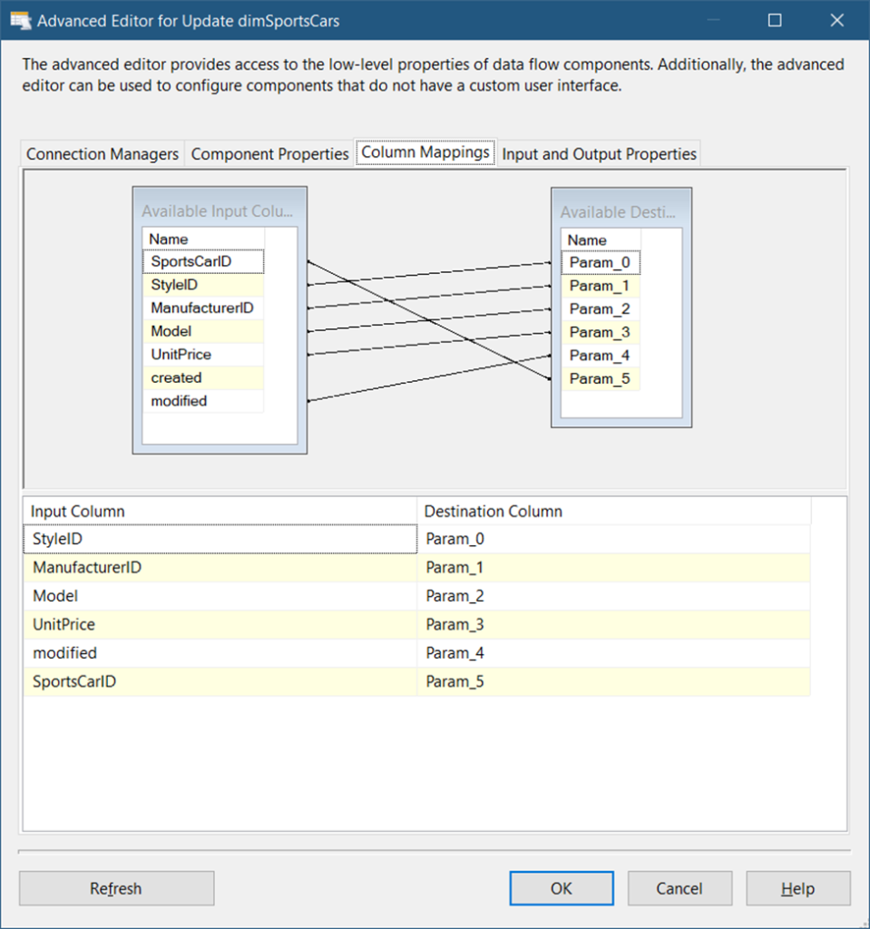
WHERE SportsCarID = ?We already did something similar earlier. The question marks are parameter placeholders. And if we map the correct source column, the corresponding target column will be set. See the mappings in Figure 29.
Finally, click OK.
D. Add an OLE DB Destination to Insert Records
This part will insert new records found in the SportsCars table into the dimSportsCars dimension table.
So, drag an OLE DB Destination component and name it Insert New Records in dimSportsCars. Double-click it and set the connection and target table. See Figure 30.
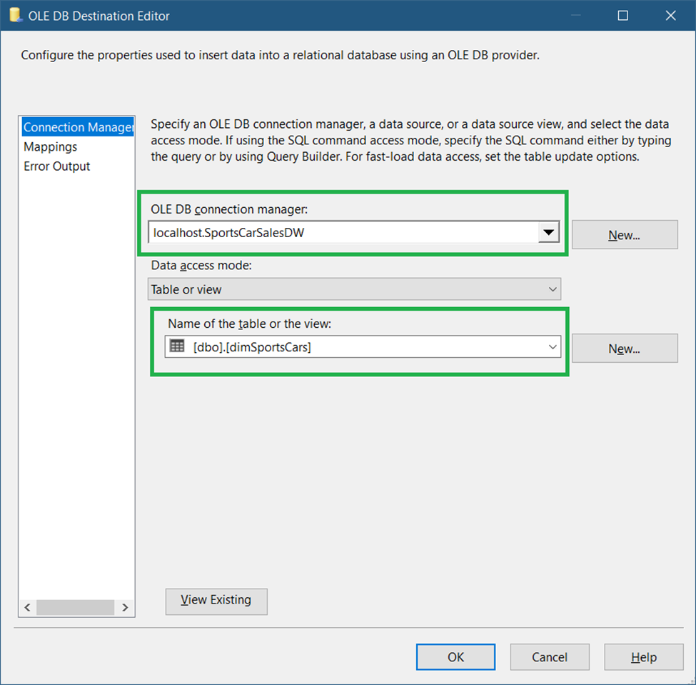
As shown in Figure 30, set the connection to the data warehouse (Figure 8) and select the dimSportsCars dimension table.
Next, click the Mappings page to see if columns are mapped accordingly. Since column names are the same in both the source and target, they will be mapped automatically.
Finally, click OK.
Package Runtime Results
Now that the package is complete, here’s a screenshot of the result in Figure 31.
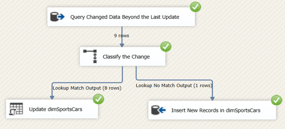
The process updated 8 rows and inserted 1 new row to the dimSportsCars dimension table.
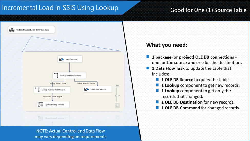
Incremental Load in SSIS Using Lookup
Another method to do incremental load is to compare the source from the target to see what needs to be inserted, updated, and deleted. And this is your option if there’s no DateTime column and no CDC on both tables. One way to do this is to use Lookup Transformation.
The typical ingredients to this approach are shown in Figure 32.
Note that the simple approach in Figure 32 is applicable for tables that do not allow hard deletes. If deletes are needed to be handled, a Merge Join using a full join may be applicable.
There are 2 subtopics for this section:
Creating the SSIS package for the SSIS incremental load using Lookup
Package runtime results
Let’s dive in.
Creating the SSIS Package for the SSIS Incremental Load Using Lookup
Our objective here is to load the rows of Manufacturers table into the dimManufacturers dimension table.
This assumes that you have a blank SSIS package ready.
The following are the summary of steps:
STEP #1. Create 2 OLE DB Connections
STEP #2. Add a Data Flow Task
Let’s begin with the example.
STEP #1. Create 2 OLE DB Connections
You can refer to Figure 19 for the source and Figure 7 for the target. We’re using the same Connection Managers here.
STEP #2. Add a Data Flow Task
Drag a Data Flow Task in the Control Flow and name it Update Manufacturers Dimension Table. Double-click it and follow the next steps. Summarized below are the steps inside the Data Flow Task.
A. Add an OLE DB Source
B. Add a Lookup Transformation to scan for new records
C. Add an OLE DB Destination to insert records.
D. Add Another Lookup Transformation to Scan for Changes
E. Add an OLE DB Command to update the target table
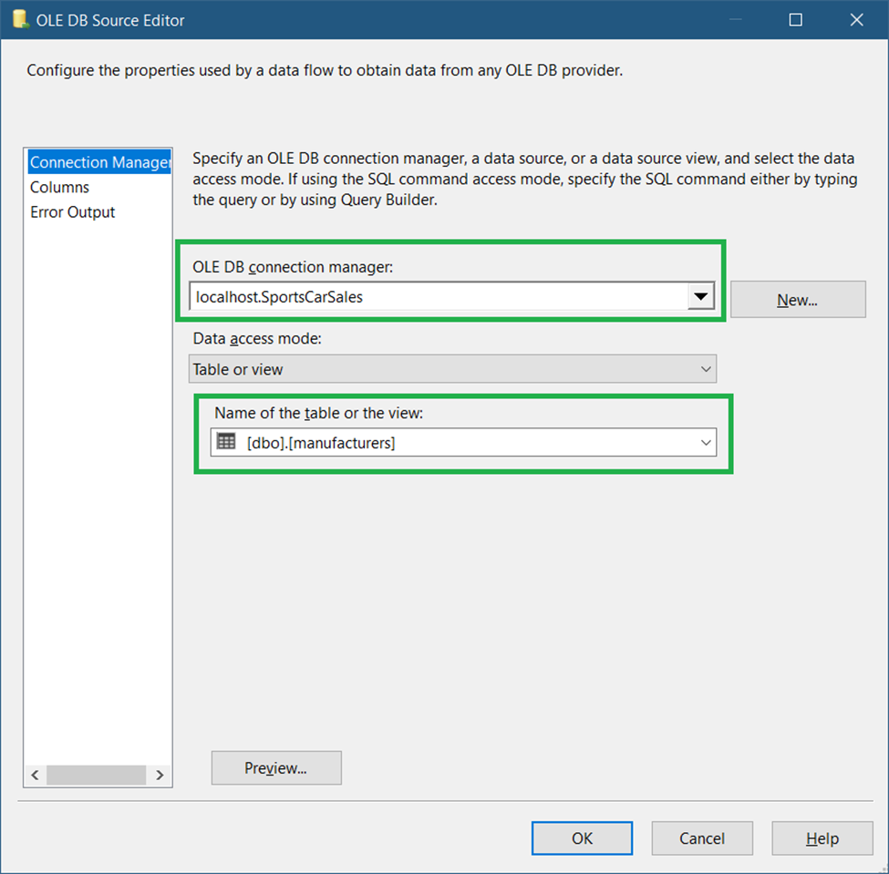
A. Add an OLE DB Source
Drag an OLE DB Source and label it Manufacturers. Set the Connection Manager as seen in Figure 33.
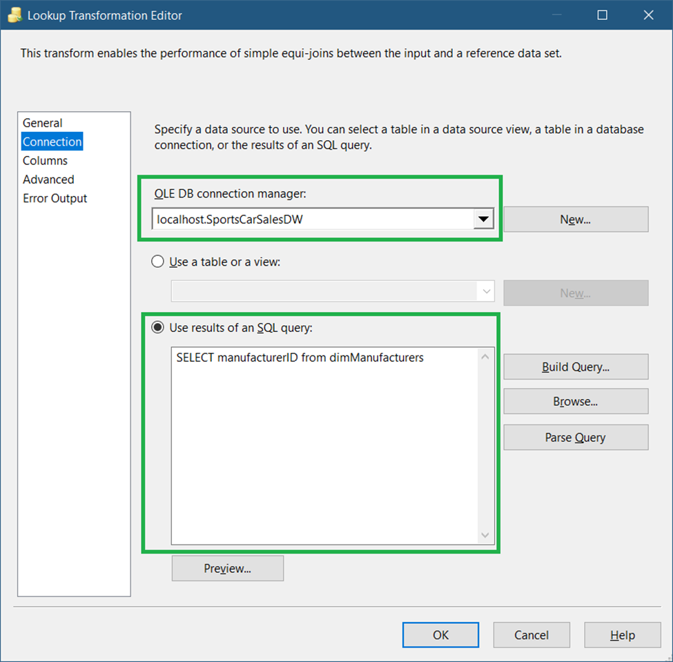
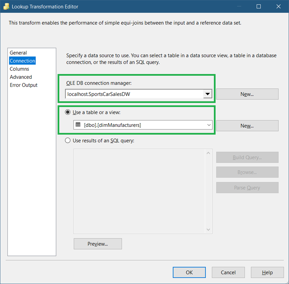
B. Add a Lookup Transformation to Scan for New Records
This Lookup Transformation will scan for records that don’t exist in the target based on the ManufacturerID key column. And all non-matching rows are candidates for table insert.
Drag a Lookup transformation and name it Lookup dimManufacturers. Then, double-click it.
The settings for the General page should be the same as in Figure 24. Meanwhile, set the connection to the data warehouse and use a query for the Connections page settings. See Figure 34.
C. Add an OLE DB Destination to Insert Records
Drag an OLE DB Destination and name it Insert New Records. Connect it to the Lookup Transformation and select Lookup No Match Output when a prompt appears. Double-click it and set the connection and target table as seen in Figure 35.
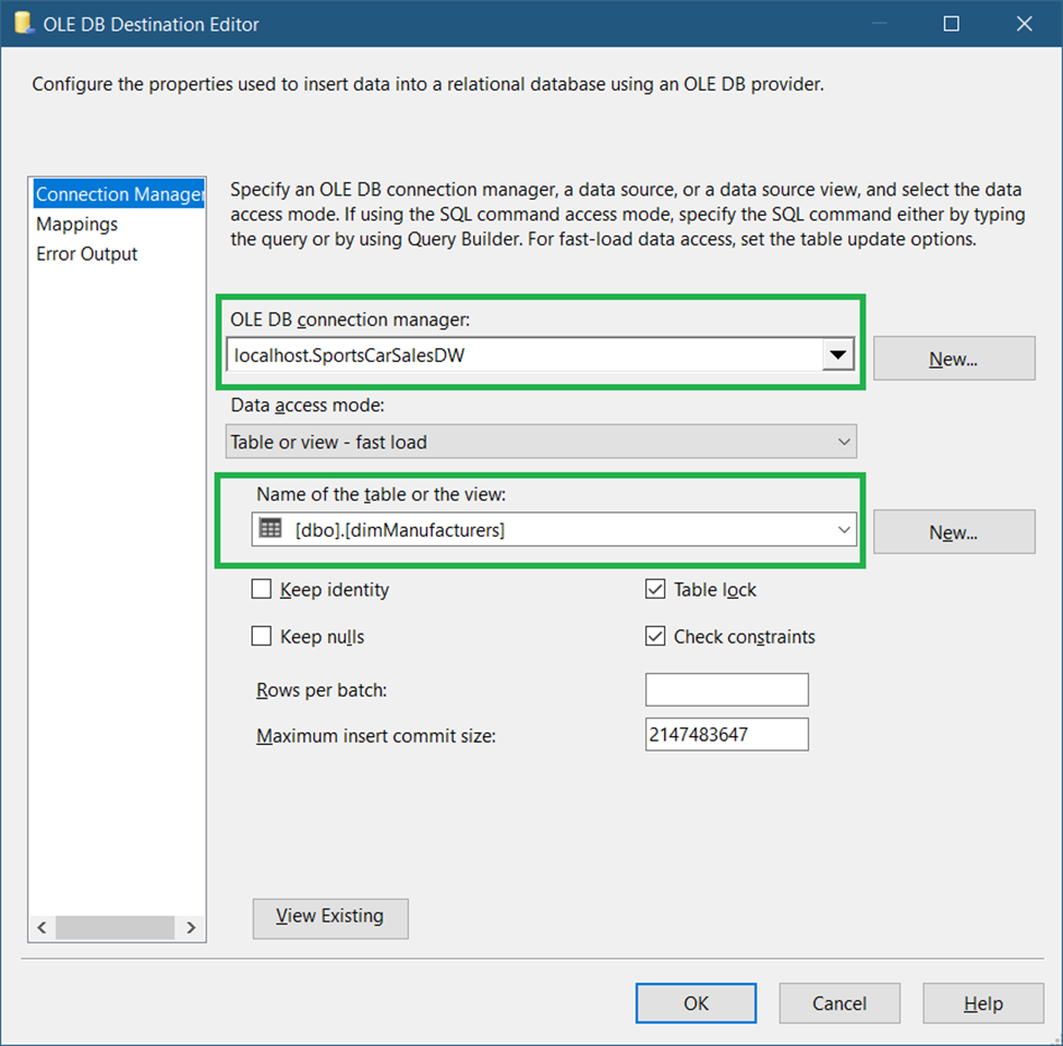
The source and target tables have the same column names and they will map automatically. See Figure 36.
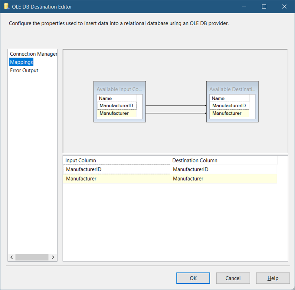
Finally, click OK.
D. Add Another Lookup Transformation to Scan for Changes
Unlike the previous Lookup Transformation, this one will scan for changes in the Manufacturer column. And if there are changes, it will be a candidate for table update.
Drag another Lookup Transformation and name it Lookup Records that Changed. Connect it to the first Lookup Transformation. The General page for this lookup should be the same as in Figure 24.
Meanwhile, the Connection page should look like Figure 37 below.
Meanwhile, notice the mappings in Figure 38.
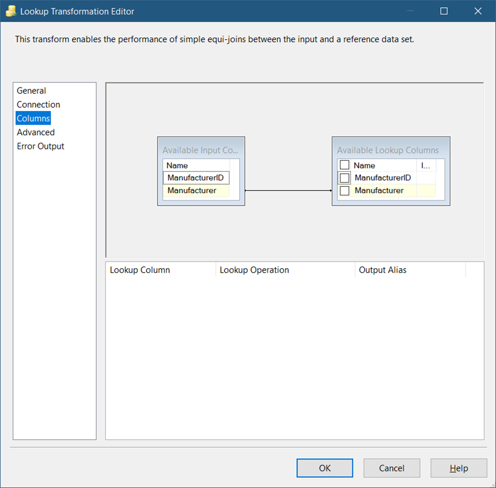
Figure 38 shows mappings through Manufacturer name. If it’s not equal, there’s a change in the source. And it needs to be copied in the target.
E. Add an OLE DB Command to Update the Target Table
The settings should be the same as in Figure 29, except for the SQLCommand. The UPDATE command should be like this:
UPDATE dimManufacturers
set manufacturer = ?
where manufacturerID = ?
Adjust the column mappings to the parameters accordingly.
Package Runtime Results
Done? Then, run the package. You will see runtime results the same as in Figure 39.
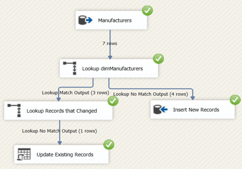
The Best Tool for SSIS Data Loading
All examples we had earlier use the out-of-the-box components that come from Microsoft. While it’s good enough for some projects, what if you have to integrate both cloud and database sources via SSIS?
This is where Devart SSIS Components come into play. These SSIS components are convenient to use. And they offer high-performance data loading using data-source-specific optimizations and advanced caching. They also have 40+ data sources, including RDBMS favorites like MySQL, PostgreSQL, and Oracle. Also included are cloud services like Salesforce, HubSpot, Google Analytics, and much more. So, it’s worth a try to load millions of records in SSIS using Devart SSIS Components.
Why not an example?
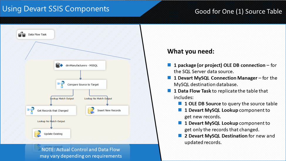
Using Devart SSIS Components to Do Incremental Load
Let’s try replicating the dimManufacturers table into MySQL, and use Devart’s Lookup and Destination components for MySQL. The recipe is shown in Figure 40.
Let’s begin by adding a new SSIS package to your Visual Studio Integration Services project. Then, add a Data Flow Task and double-click it. Then, follow the steps below.
Before that, here’s a summary of the steps:
STEP #1. Add an OLE DB Source
STEP #2. Add a Devart MySQL Connection Manager
STEP #3. Add a Devart MySQL Lookup to scan for new records
STEP #4. Add another Devart MySQL Lookup Transformation to scan for changes
STEP #5. Add a Devart MySQL Destination to insert records
STEP #6. Add another Devart MySQL Destination to update records
STEP #1. Add an OLE DB Source
This will connect to the SQL Server database we had earlier. Please refer to Figure 8. Then, set the table to dimManufacturers.
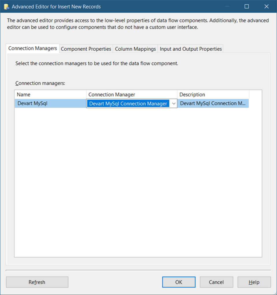
STEP #2. Add a Devart MySQL Connection Manager
We need this connection for the destination database and table. So, in the Connection Managers window, right-click and select New Connection. Then, select the DevartMySQL Connection Manager type. Then, configure the database access as shown in Figure 41. Notice the simpler interface to connect. Though you can go to the Advanced tab and see more properties there.
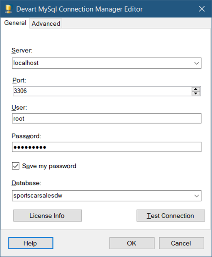
I’m running MySQL 8 in my local machine and there’s a copy of the same database in SQL Server, but the rows are older.
STEP #3. Add a Devart MySQL Lookup Transformation to Scan for New Records
Drag a Devart MySQL Lookup and name it Compare Source to Target. Then, connect it to the Devart MySQL Connection Manager earlier. Now, follow the configuration in Figure 42.
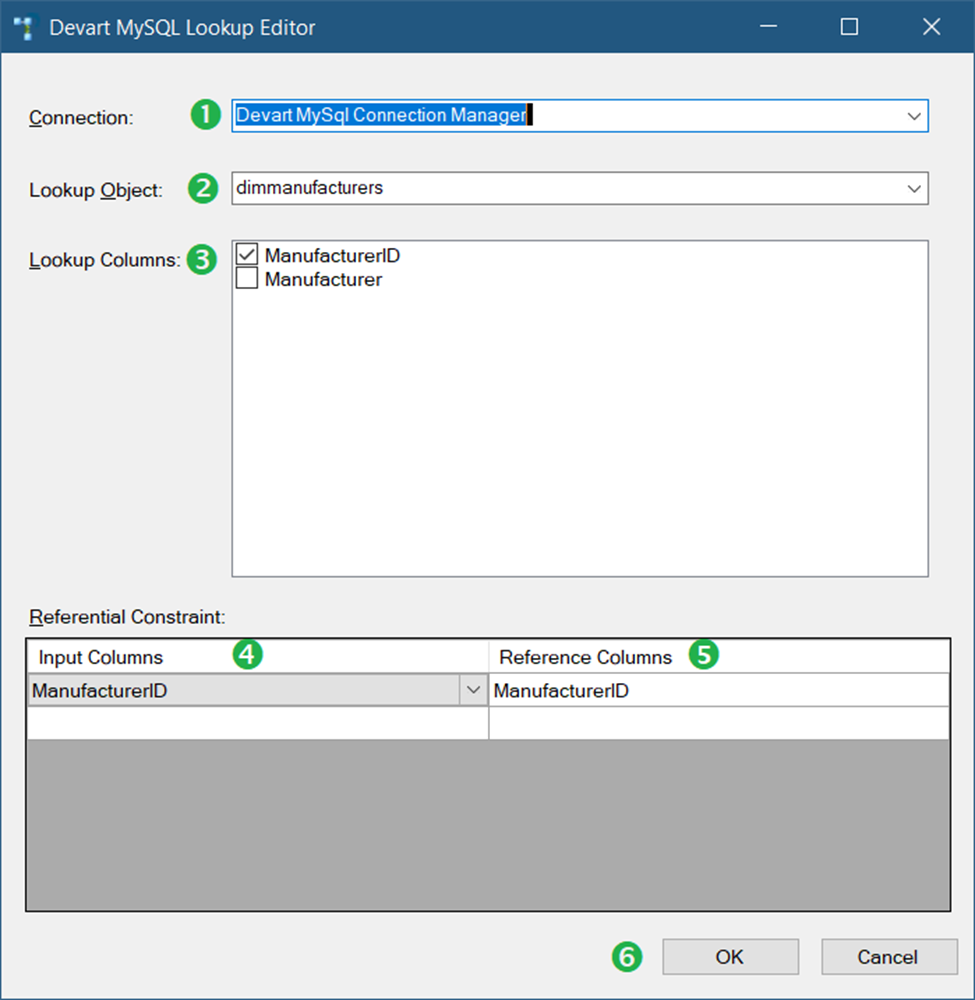
Following the numbers in Figure 42, the following are the details:
- First, select the Devart MySQL Connection Manager created in STEP #2.
- Then, select the dimmanufacturers table.
- In Lookup Columns, mark checked the ManufacturerID column.
- Then, in Input Columns, select ManufacturerID.
- Then, select ManufacturerID in Reference Columns.
- Finally, click OK.
NOTE: If you encounter a duplicate name error, go to Advanced Editor. And then, click Input and Output Properties. Rename either the Input or Output Column to a different name.
STEP #4. Add another Devart MySQL Lookup Transformation to Scan for Changes
This second MySQL Lookup will scan for records that changed.
Drag another Devart MySQL Lookup and label it Get Records that Changed. Connect it to the first Devart MySQL Lookup. Then, choose Lookup Match Output.
The setup is the same as in Figure 42. But choose the Manufacturer column instead of ManufacturerID. Do this for Lookup Columns, Input Columns, and Reference Columns.
STEP #5. Add a Devart MySQL Destination to Insert Records
This step will insert records from the source that have no match in the target.
So, drag a Devart MySQL Destination and label it Insert New Records. Connect it to the first Devart MySQL Lookup. Double-click it and configure the Connection Manager. See Figure 43.
In Figure 43, you need to set the connection to the MySQL connection manager we did in STEP #2. Then, click Component Properties. See the configuration in Figure 44.
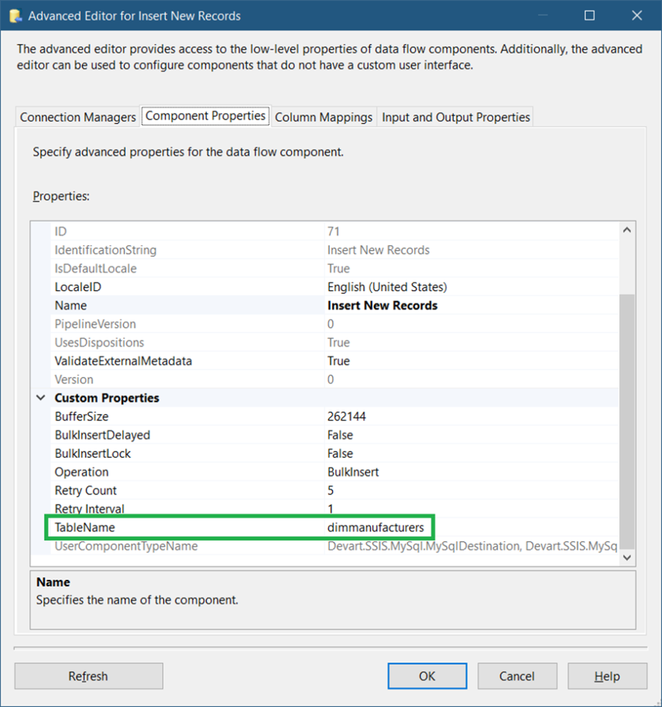
After setting the TableName to dimmanufacturers, click Column Mappings. Since both the source and target tables have the same column names, the columns are automatically mapped.
Finally, click OK.
STEP #6. Add Another Devart MySQL Destination to Update Records
Unlike the other Devart MySQL Destination, this will update records that changed from the source.
So, drag another Devart MySQL Destination and label it Update Existing. Connect it to the second Devart MySQL Lookup Transformation. And select Lookup No Match Output when a prompt appears. The setup is the same as in STEP #5 except for the Component Properties. See Figure 45 on what to change.
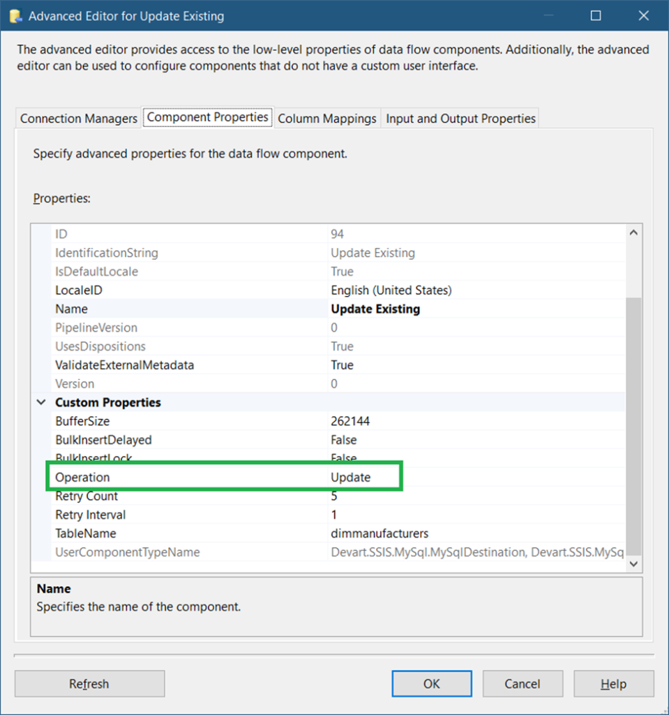
Using the Devart MySQL Destination is dead easy than using an OLE DB Command. There’s no need to map parameters to columns. It also works for a Delete operation. This is unlike an OLE DB Destination that works for inserts only.
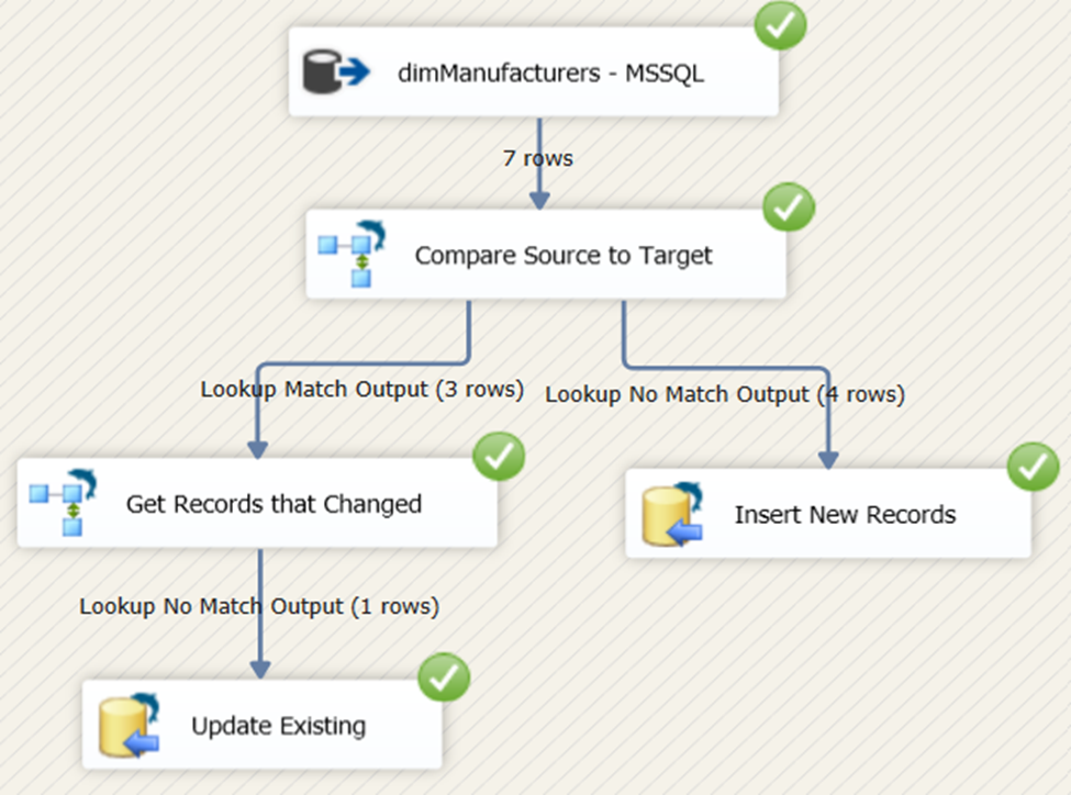
Package Runtime Results
See the runtime results in Figure 46.
Conclusion
That’s it.
You learned 3 ways to do incremental load in SSIS by using the following:
- Change Data Capture
- DateTime Columns
- Lookup Transformation
You also learned how to do it using Devart SSIS Components.
Though our examples are simplified to make the principle easier to understand as possible, there’s room for improvement. We didn’t use a staging table to store all changes, whether insert, update, or delete. This is recommended for very large data, especially when the target is in another server. You can also add an execute process task in SSIS for special scenarios.
Anyway, if you like this post, please share it on your favorite social media platforms.